Simple data mining examples and datasets
See data mining examples, including examples of data mining algorithms and simple datasets, that will help you learn how data mining works and how companies can make data-related decisions based on set rules.
 Data Mining: Know it All
This excerpt from Data Mining: Know It All includes examples that show how data mining algorithms and datasets work. Learn how companies can make data-related decisions based on set rules.
1.2 Simple Examples: The Weather Problem and Others
We use a lot of examples in this book, which seems particularly appropriate considering that the book is all about learning from examples! There are several standard datasets that we will come back to repeatedly. Different datasets tend to expose new issues and challenges, and it is interesting and instructive to have in mind a variety of problems when considering learning methods. In fact, the need to work with different datasets is so important that a corpus containing around 100 example problems has been gathered together so that different algorithms can be tested and compared on the same set of problems.
Table of contents:
An introduction to data mining
Simple data mining examples and datasets
Fielded applications of data mining and machine learning
The difference between machine learning and statistics in data mining
Information and examples on data mining and ethics
Data acquisition and integration techniques
What is a data rollup?
Calculating mode in data mining projects
Using data merging and concatenation techniques to integrate data
The illustrations used here are all unrealistically simple. Serious application of data mining involves thousands, hundreds of thousands, or even millions of individual cases. But when explaining what algorithms do and how they work, we need simple examples that capture the essence of the problem but are small enough to be comprehensible in every detail. The illustrations we will be working with are intended to be "academic" in the sense that they will help us to understand what is going on. Some actual fielded applications of learning techniques are discussed in Section 1.3, and many more are covered in the books mentioned in the Further Reading section at the end of the chapter.
Copyright info
Printed with permission from Morgan Kaufmann, a division of Elsevier. Copyright 2009. Data Mining: Know It All by Chakrabarti, et al. For more information about this title and other similar books, please visit www.elsevierdirect.com.
Another problem with actual real-life datasets is that they are often proprietary. No corporation is going to share its customer and product choice database with you so that you can understand the details of its data mining application and how it works. Corporate data is a valuable asset, one whose value has increased enormously with the development of data mining techniques such as those described in this book. Yet we are concerned here with understanding how the methods used for data mining work and understanding the details of these methods so that we can trace their operation on actual data. That is why our illustrations are simple ones. But they are not simplistic: they exhibit the features of real datasets.
1.2.1 The Weather Problem
The weather problem is a tiny dataset that we will use repeatedly to illustrate machine learning methods. Entirely fictitious, it supposedly concerns the conditions that are suitable for playing some unspecified game. In general, instances in a dataset are characterized by the values of features, or attributes, that measure different aspects of the instance. In this case there are four attributes: outlook, temperature, humidity, and windy. The outcome is whether or not to play.
In its simplest form, shown in Table 1.2 , all four attributes have values that are symbolic categories rather than numbers. Outlook can be sunny, overcast, or rainy; temperature can be hot, mild, or cool; humidity can be high or normal; and windy can be true or false. This creates 36 possible combinations (3 X 3 X 2 X 2 = 36), of which 14 are present in the set of input examples.
A set of rules learned from this information -- not necessarily a very good one -- might look as follows:
| If outlook = sunny and humidity = high | then play = no |
| If outlook = rainy and windy = true | then play = no |
| If outlook = overcast | then play = yes |
| If humidity = normal | then play = yes |
| If none of the above | then play = yes |
These rules are meant to be interpreted in order: the first one; then, if it doesn't apply, the second; and so on.
A set of rules intended to be interpreted in sequence is called a decision list. Interpreted as a decision list, the rules correctly classify all of the examples in the table, whereas taken individually, out of context, some of the rules are incorrect. For example, the rule if humidity = normal, then play = yes gets one of the examples wrong (check which one). The meaning of a set of rules depends on how it is interpreted -- not surprisingly!
Learn about the new ethical dilemmas posed by the growing power of analytics
Find out how NASA has used text analytics to improve aviation safety
Read about the need for open organizational minds in predictive analytics programs
In the slightly more complex form shown in Table 1.3, two of the attributes -- temperature and humidity -- have numeric values. This means that any learning method must create inequalities involving these attributes rather than simple equality tests, as in the former case. This is called a numeric-attribute problem -- in this case, a mixed-attribute problem because not all attributes are numeric.
Now the first rule given earlier might take the following form:
If outlook = sunny and humidity > 83 then play = no
A slightly more complex process is required to come up with rules that involve numeric tests.
Table 1.2 The Weather Data
| Outlook | Temperature | Humidity | Windy | Play |
| Sunny | Hot | High | False | No |
| Sunny | Hot | High | True | No |
| Overcast | Hot | High | False | Yes |
| Rainy | Mild | High | False | Yes |
| Rainy | Cool | Normal | False | Yes |
| Rainy | Cool | Normal | True | No |
| Overcast | Cool | Normal | True | Yes |
| Sunny | Mild | High | False | No |
| Sunny | Cool | Normal | False | Yes |
| Rainy | Mild | Normal | False | Yes |
| Sunny | Mild | Normal | True | Yes |
| Overcast | Mild | High | True | Yes |
| Overcast | Hot | Normal | False | Yes |
| Rainy | Mild | High | True | No |
The rules we have seen so far are classification rules: they predict the classification of the example in terms of whether or not to play. It is equally possible to disregard the classification and just look for any rules that strongly associate different attribute values. These are called association rules. Many association rules can be derived from the weather data in Table 1.2. Some good ones are as follows:
| If temperature = cool | then humidity = normal |
| If humidity = normal and windy = false | then play = yes |
| If outlook = sunny and play = no | then humidity = high |
| If windy = false and play = no | then outlook = sunny and humidity = high. |
Table 1.3 Weather Data with Some Numeric Attribute
| Outlook | Temperature | Humidity | Windy | Play |
| Sunny | 85 | 85 | False | No |
| Sunny | 80 | 90 | True | No |
| Overcast | 83 | 86 | False | Yes |
| Rainy | 70 | 96 | False | Yes |
| Rainy | 68 | 80 | False | Yes |
| Rainy | 65 | 70 | True | No |
| Overcast | 64 | 65 | True | Yes |
| Sunny | 72 | 95 | False | No |
| Sunny | 69 | 70 | False | Yes |
| Rainy | 75 | 80 | False | Yes |
| Sunny | 75 | 70 | True | Yes |
| Overcast | 72 | 90 | True | Yes |
| Overcast | 81 | 75 | False | Yes |
| Rainy | 71 | 91 | True | No |
All these rules are 100 percent correct on the given data; they make no false predictions. The first two apply to four examples in the dataset, the third to three examples, and the fourth to two examples. There are many other rules: in fact, nearly 60 association rules can be found that apply to two or more examples of the weather data and are completely correct on this data. If you look for rules that are less than 100 percent correct, then you will find many more. There are so many because unlike classification rules, association rules can "predict" any of the attributes, not just a specified class, and can even predict more than one thing. For example, the fourth rule predicts both that outlook will be sunny and that humidity will be high.
1.2.2 Contact Lenses: An Idealized Problem
The contact lens data introduced earlier tells you the kind of contact lens to prescribe, given certain information about a patient. Note that this example is intended for illustration only: it grossly oversimplifies the problem and should certainly not be used for diagnostic purposes!
The first column of Table 1.1 gives the age of the patient. In case you're wondering, presbyopia is a form of longsightedness that accompanies the onset of middle age. The second gives the spectacle prescription: myope means shortsighted and hypermetrope means longsighted. The third shows whether the patient is astigmatic, and the fourth relates to the rate of tear production, which is important in this context because tears lubricate contact lenses. The final column shows which kind of lenses to prescribe: hard, soft, or none. All possible combinations of the attribute values are represented in the table.
A sample set of rules learned from this information is shown in Figure 1.1 . This is a large set of rules, but they do correctly classify all the examples. These rules are complete and deterministic: they give a unique prescription for every conceivable example. Generally, this is not the case. Sometimes there are situations in which no rule applies; other times more than one rule may apply, resulting in conflicting recommendations. Sometimes probabilities or weights may be associated with the rules themselves to indicate that some are more important, or more reliable, than others.
You might be wondering whether there is a smaller rule set that performs as well. If so, would you be better off using the smaller rule set and, if so, why? These are exactly the kinds of questions that will occupy us in this book. Because the examples form a complete set for the problem space, the rules do no more than summarize all the information that is given, expressing it in a different and more concise way. Even though it involves no generalization, this is often a useful thing to do! People frequently use machine learning techniques to gain insight into the structure of their data rather than to make predictions for new cases. In fact, a prominent and successful line of research in machine learning began as an attempt to compress a huge database of possible chess endgames and their outcomes into a data structure of reasonable size. The data structure chosen for this enterprise was not a set of rules, but a decision tree.
Figure 1.1. Rules for the contact lenses data
| If tear production rate = reduced then recommendation = none If age = young and astigmatic = no and tear production rate = normal then recommendation = soft If age = pre-presbyopic and astigmatic = no and tear production rate = normal then recommendation = soft If age = presbyopic and spectacle prescription = myope and astigmatic = no then recommendation = none If spectacle prescription = hypermetrope and astigmatic = no and tear production rate = normal then recommendation = soft If spectacle prescription = myope and astigmatic = yes and tear production rate = normal then recommendation = hard If age = young and astigmatic = yes and tear production rate = normal then recommendation = hard If age = pre-presbyopic and spectacle prescription = hypermetrope and astigmatic = yes then recommendation = none If age = presbyopic and spectacle prescription = hypermetrope and astigmatic = yes then recommendation = none |
Figure 1.2. Decision tree for the contact lenses data
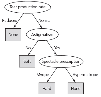
Figure 1.2 presents a structural description for the contact lens data in the form of a decision tree, which for many purposes is a more concise and perspicuous representation of the rules and has the advantage that it can be visualized more easily. (However, this decision tree -- in contrast to the rule set given in Figure 1.1 -- classifies two examples incorrectly.) The tree calls first for a test on tear production rate, and the first two branches correspond to the two possible outcomes. If tear production rate is reduced (the left branch), the outcome is none. If it is normal (the right branch), a second test is made, this time on astigmatism. Eventually, whatever the outcome of the tests, a leaf of the tree is reached that dictates the contact lens recommendation for that case.
1.2.3 Irises: A Classic Numeric Dataset
The iris dataset, which dates back to seminal work by the eminent statistician R. A. Fisher in the mid-1930s and is arguably the most famous dataset used in data mining, contains 50 examples each of three types of plant: Iris setosa, Iris versicolor, and Iris virginica. It is excerpted in Table 1.4. There are four attributes: sepal length, sepal width, petal length, and petal width (all measured in centimeters). Unlike previous datasets, all attributes have numeric values.
Table 1.4 The Iris Data
| Sepal Length (cm) | Sepal Width (cm) | Petal Length (cm) | Petal Width (cm) | Type | ||||||
| 1 | 5.1 | 3.5 | 1.4 | 0.2 | Iris setosa | |||||
| 2 | 4.9 | 3.0 | 1.4 | 0.2 | Iris setosa | |||||
| 3 | 4.7 | 3.2 | 1.3 | 0.2 | Iris setosa | |||||
| 4 | 4.6 | 3.1 | 1.5 | 0.2 | Iris setosa | |||||
| 5 | 5.0 | 3.6 | 1.4 | 0.2 | Iris setosa | |||||
| … | ||||||||||
| 51 | 7.0 | 3.2 | 4.7 | 1.4 | Iris versicolor | |||||
| 52 | 6.4 | 3.2 | 4.5 | 1.5 | Iris versicolor | |||||
| 53 | 6.9 | 3.1 | 4.9 | 1.5 | Iris versicolor | |||||
| 54 | 5.5 | 2.3 | 4.0 | 1.3 | Iris versicolor | |||||
| 55 | 6.5 | 2.8 | 4.6 | 1.5 | Iris versicolor | |||||
| … | ||||||||||
| 101 | 6.3 | 3.3 | 6.0 | 2.5 | Iris virginica | |||||
| 102 | 5.8 | 2.7 | 5.1 | 1.9 | Iris virginica | |||||
| 103 | 7.1 | 3.0 | 5.9 | 2.1 | Iris virginica | |||||
| 104 | 6.3 | 2.9 | 5.6 | 1.8 | Iris virginica | |||||
| 105 | 6.5 | 3.0 | 5.8 | 2.2 | Iris virginica | |||||
| … | ||||||||||
The following set of rules might be learned from this dataset:
If petal length < 2.45 then Iris setosa
If sepal width < 2.10 then Iris versicolor
If sepal width < 2.45 and petal length < 4.55 then Iris versicolor
If sepal width < 2.95 and petal width < 1.35 then Iris versicolor
If petal length ≥ 2.45 and petal length < 4.45 then Iris versicolor
If sepal length ≥ 5.85 and petal length < 4.75 then Iris versicolor
If sepal width < 2.55 and petal length < 4.95 and
petal width < 1.55 then Iris versicolor
If petal length ≥2.45 and petal length < 4.95 and
petal width < 1.55 then Iris versicolor
If sepal length ≥ 6.55 and petal length < 5.05 then Iris versicolor
If sepal width < 2.75 and petal width < 1.65 and
sepal length < 6.05 then Iris versicolor
If sepal length ≥5.85 and sepal length < 5.95 and
petal length < 4.85 then Iris versicolor
If petal length ≥ 5.15 then Iris virginica
If petal width ≥1.85 then Iris virginica
If petal width ≥ 1.75 and sepal width < 3.05 then Iris virginica
If petal length ≥ 4.95 and petal width < 1.55 then Iris virginica
These rules are very cumbersome; more compact rules can be expressed that convey the same information.
1.2.4 CPU Performance: Introducing Numeric Prediction
Although the iris dataset involves numeric attributes, the outcome -- the type of iris -- is a category, not a numeric value. Table 1.5 shows some data for which the outcome and the attributes are numeric. It concerns the relative performance of computer processing power on the basis of a number of relevant attributes; each row represents 1 of 209 different computer configurations.
The classic way of dealing with continuous prediction is to write the outcome as a linear sum of the attribute values with appropriate weights, for example:
- 0.2700 CHMIN + 1.480 CHMAX
Table 1.5 The CPU Performance Data
| Cycle Time (ns) MYCT | Main Memory (KB) | Cache (KB) CACH | Channels | Performance PRP | ||||||||
| Minimum MMN | Maximum MMAX | Minimum CHMIN | Maximum CHMAX | |||||||||
| 1 | 125 | 256 | 6000 | 256 | 16 | 128 | 198 | |||||
| 2 | 29 | 8000 | 32000 | 32 | 8 | 32 | 269 | |||||
| 3 | 29 | 8000 | 32000 | 32 | 8 | 32 | 220 | |||||
| 4 | 29 | 8000 | 32000 | 32 | 8 | 32 | 172 | |||||
| 5 | 29 | 8000 | 16000 | 32 | 8 | 16 | 132 | |||||
| … | ||||||||||||
| 207 | 126 | 2000 | 8000 | 0 | 2 | 14 | 52 | |||||
| 208 | 480 | 512 | 8000 | 32 | 0 | 0 | 67 | |||||
| 209 | 480 | 1000 | 4000 | 0 | 0 | 0 | 45 | |||||
(The abbreviated variable names are given in the second row of the table.) This is called a regression equation, and the process of determining the weights is called regression, a well-known procedure in statistics. However, the basic regression method is incapable of discovering nonlinear relationships (although variants do exist).
In the iris and central processing unit (CPU) performance data, all the attributes have numeric values. Practical situations frequently present a mixture of numeric and nonnumeric attributes.
1.2.5 Labor Negotiations: A More Realistic Example
The labor negotiations dataset in Table 1.6 summarizes the outcome of Canadian contract negotiations in 1987 and 1988. It includes all collective agreements reached in the business and personal services sector for organizations with at least 500 members (teachers, nurses, university staff, police, etc.). Each case concerns one contract, and the outcome is whether the contract is deemed acceptable or unacceptable. The acceptable contracts are ones in which agreements were accepted by both labor and management. The unacceptable ones are either known offers that fell through because one party would not accept them or acceptable contracts that had been significantly perturbed to the extent that, in the view of experts, they would not have been accepted.
Table 1.6 The Labor Negotiations Data
| Attribute | Type | 1 | 2 | 3 | … | 40 |
| Duration | Years | 1 | 2 | 3 | 2 | |
| Wage increase first year | Percentage | 2% | 4% | 4.3% | 4.5 | |
| Wage increase second year | Percentage | ? | 5% | 4.4% | 4.0 | |
| Wage increase third year | Percentage | ? | ? | ? | ? | |
| Cost of living adjustment | [none, tcf, tc] | None | TCF | ? | None | |
| Working hours per week | Hours | 28 | 35 | 38 | 40 | |
| Pension | [none, ret-allw, empl-cntr] | None | ? | ? | ? | |
| Standby pay | Percentage | ? | 13% | ? | ? | |
| Shift-work supplement | Percentage | ? | 5% | 4% | 4% | |
| Education allowance | [yes, no] | Yes | ? | ? | ? | |
| Statutory holidays | Days | 11 | 15 | 12 | 12 | |
| Vacation | [below-avg, avg, gen] | Avg | Gen | Gen | Avg | |
| Long-term disability insurance | [yes, no] | No | ? | ? | Yes | |
| Dental plan contribution | [none, half, full] | None | ? | Full | Full | |
| Bereavement assistance | [yes, no] | No | ? | ? | Yes | |
| Health plan contribution | [none, half, full] | None | ? | Full | Half | |
| Acceptability of contract | [good, bad] | Bad | Good | Good | Good |
There are 40 examples in the dataset (plus another 17 that are normally reserved for test purposes). Unlike the other tables here, Table 1.6 presents the examples as columns rather than as rows; otherwise, it would have to be stretched over several pages. Many of the values are unknown or missing, as indicated by question marks.
This is a much more realistic dataset than the others we have seen. It contains many missing values, and it seems unlikely that an exact classification can be obtained.
Figure 1.3 shows two decision trees that represent the dataset. Figure 1.3(a) is simple and approximate: it doesn't represent the data exactly. For example, it will predict bad for some contracts that are actually marked good. But it does make intuitive sense: a contract is bad (for the employee!) if the wage increase in the first year is too small (less than 2.5 percent). If the first-year wage increase is larger than this, it is good if there are lots of statutory holidays (more than 10 days). Even if there are fewer statutory holidays, it is good if the first-year wage increase is large enough (more than 4 percent).
Figure 1.3(b) is a more complex decision tree that represents the same dataset. In fact, this is a more accurate representation of the actual dataset that was used to create the tree. But it is not necessarily a more accurate representation of the underlying concept of good versus bad contracts. Look down the left branch. It doesn't seem to make sense intuitively that, if the working hours exceed 36, a contract is bad if there is no health-plan contribution or a full health-plan contribution but is good if there is a half health-plan contribution. It is certainly reasonable that the health-plan contribution plays a role in the decision but not if half is good and both full and none are bad. It seems likely that this is an artifact of the particular values used to create the decision tree rather than a genuine feature of the good versus bad distinction.
The tree in Figure 1.3(b) is more accurate on the data that was used to train the classifier but will probably perform less well on an independent set of test data. It is "overfitted" to the training data -- it follows it too slavishly. The tree in Figure 1.3(a) is obtained from the one in Figure 1.3(b) by a process of pruning.
1.2.6 Soybean Classification: A Classic Machine Learning Success
An often-quoted early success story in the application of machine learning to practical problems is the identification of rules for diagnosing soybean diseases. 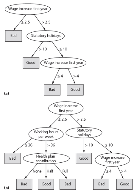
The data is taken from questionnaires describing plant diseases. There are about 680 examples, each representing a diseased plant. Plants were measured on 35 attributes, each one having a small set of possible values. Examples are labeled with the diagnosis of an expert in plant biology: there are 19 disease categories altogether -- horrible-sounding diseases, such as diaporthe stem canker, rhizoctonia root rot, and bacterial blight, to mention just a few.
More on data mining:
- Continue to the next section: Fielded applications of data mining and machine learning
- Download a PDF of this chapter for free: "What's It All About?"
- Read other excerpts from data management books in the Chapter Download Library.
Table 1.7 gives the attributes, the number of different values that each can have, and a sample record for one particular plant. The attributes are placed into different categories just to make them easier to read.
Here are two example rules, learned from this data:
If [leaf condition is normal and
stem condition is abnormal and
stem cankers is below soil line and
canker lesion color is brown]
then
diagnosis is rhizoctonia root rot
If [leaf malformation is absent and
stem condition is abnormal and
stem cankers is below soil line and
canker lesion color is brown]
then
diagnosis is rhizoctonia root rot
These rules nicely illustrate the potential role of prior knowledge -- often called domain knowledge -- in machine learning, because the only difference between the two descriptions is leaf condition is normal versus leaf malformation is absent. In this domain, if the leaf condition is normal, then leaf malformation is necessarily absent, so one of these conditions happens to be a special case of the other. Thus, if the first rule is true, the second is necessarily true as well. The only time the second rule comes into play is when leaf malformation is absent but leaf condition is not normal -- that is, when something other than malformation is wrong with the leaf. This is certainly not apparent from a casual reading of the rules.
Table 1.7 The Soybean Data
| Attribute | |||
| Number of Values | Sample Value | ||
| Environment | Time of occurrence | 7 | July |
| Precipitation | 3 | Above normal | |
| Temperature | 3 | Normal | |
| Cropping history | 4 | Same as last year | |
| Hail damage | 2 | Yes | |
| Damaged area | 4 | Scattered | |
| Severity | 3 | Severe | |
| Plant height | 2 | Normal | |
| Plant growth | 2 | Abnormal | |
| Seed treatment | 3 | Fungicide | |
| Germination | 3 | Less than 80% | |
| Seed | Condition | 2 | Normal |
| Mold growth | 2 | Absent | |
| Discoloration | 2 | Absent | |
| Size | 2 | Normal | |
| Shriveling | 2 | Absent | |
| Fruit | Condition of fruit pods | 3 | Normal |
| Fruit spots | 5 | --- | |
| Leaf | Condition | 2 | Abnormal |
| Leaf spot size | 3 | --- | |
| Yellow leaf spot halo | 3 | Absent | |
| Leaf spot margins | 3 | --- | |
| Shredding | 2 | Absent | |
| Leaf malformation | 2 | Absent | |
| Leaf mildew growth | 3 | Absent | |
| Stem | Condition | 2 | Abnormal |
| Stem lodging | 2 | Yes | |
| Stem cankers | 4 | Above soil line | |
| Canker lesion color | 3 | --- | |
| Fruiting bodies on stems | 2 | Present | |
| External decay of stem | 3 | Firm and dry | |
| Mycelium on stem | 2 | Absent | |
| Internal discoloration | 3 | None | |
| Sclerotia | 2 | Absent | |
| Root | Condition | 3 | Normal |
| Diagnosis | Diaporthe stem | ||
| 19 | Canker |
Research on this problem in the late 1970s found that these diagnostic rules could be generated by a machine learning algorithm, along with rules for every other disease category, from about 300 training examples. The examples were carefully selected from the corpus of cases as being quite different from one another -- "far apart" in the example space. At the same time, the plant pathologist who had produced the diagnoses was interviewed, and his expertise was translated into diagnostic rules. Surprisingly, the computer-generated rules outperformed the expert's rules on the remaining test examples. They gave the correct disease top ranking 97.5 percent of the time compared with only 72 percent for the expert-derived rules. Furthermore, not only did the learning algorithm find rules that outperformed those of the expert collaborator, but the same expert was so impressed that he allegedly adopted the discovered rules in place of his own!